Excitation function

This example demonstrates the use of various excitation functions provided by the pymycar.VerticalModels.exitations module. These functions are commonly used to simulate inputs in vertical dynamics models of vehicles.

The following excitation functions are illustrated:

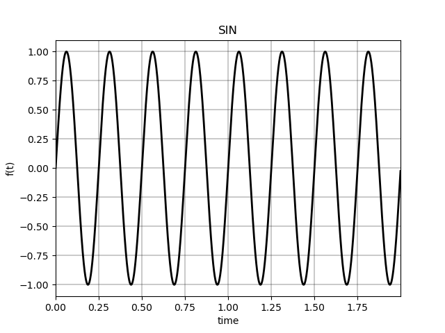
• SIN Excitation: A simple sinusoidal excitation function.

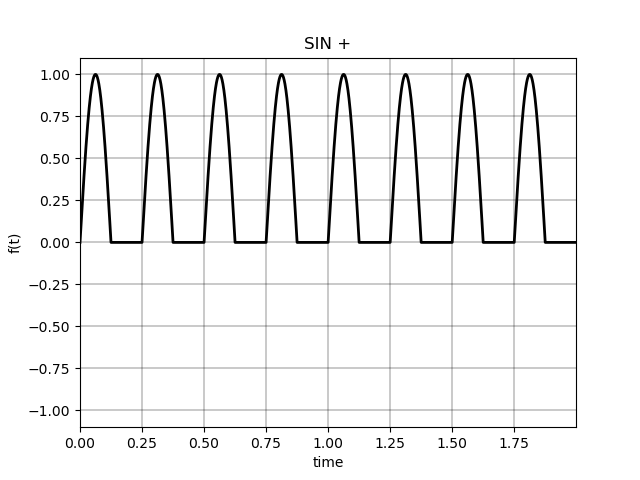
• SIN+ Excitation: The positive part of a sinusoidal excitation function.

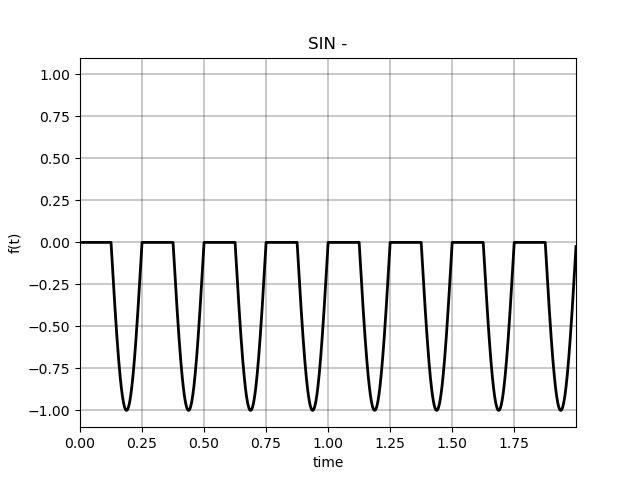
• SIN- Excitation: The negative part of a sinusoidal excitation function.

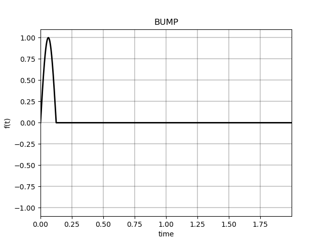
• BUMP Excitation: A single bump excitation function.

Each excitation function is plotted over a time interval, demonstrating how the signal evolves.

Import necessary libraries

import matplotlib.pyplot as plt
import numpy as np

Import from pymycar package

from pymycar.VerticalModels.exitations import (
    sin_exitation,
    sin_possitive_part_exitation,
    sin_negative_part_exitation,
    bump_exitation,
)

#%
# An amplitude of 1 and a frequency of 4 are used.
amplitude = 1
frequency = 4
t = np.arange(0, 2, 0.001)

SIN excitation function

Create a subplot for the SIN excitation function

fig, ax_sin = plt.subplots()
ax_sin.plot(t, sin_exitation(t, amplitude, frequency), 'k-', linewidth=2.0)
ax_sin.grid(color='k', linestyle='-', linewidth=0.3)
ax_sin.set_xlabel('time')
ax_sin.set_ylabel('f(t)')
ax_sin.set_title('SIN')
ax_sin.set_xlim(np.min(t), np.max(t))
ax_sin.set_ylim(-amplitude*1.1, amplitude*1.1)

(-1.1, 1.1)

SIN + excitation function

Create a subplot for the SIN + excitation function

fig, ax_sinposs = plt.subplots()
ax_sinposs.plot(t, sin_possitive_part_exitation(t, amplitude, frequency), 'k-', linewidth=2.0)
ax_sinposs.grid(color='k', linestyle='-', linewidth=0.3)
ax_sinposs.set_xlabel('time')
ax_sinposs.set_ylabel('f(t)')
ax_sinposs.set_title('SIN +')
ax_sinposs.set_xlim(np.min(t), np.max(t))
ax_sinposs.set_ylim(-amplitude*1.1, amplitude*1.1)

(-1.1, 1.1)

SIN - excitation function

Create a subplot for the SIN - excitation function

fig, ax_sinneg = plt.subplots()
ax_sinneg.plot(t, sin_negative_part_exitation(t, amplitude, frequency), 'k-', linewidth=2.0)
ax_sinneg.grid(color='k', linestyle='-', linewidth=0.3)
ax_sinneg.set_xlabel('time')
ax_sinneg.set_ylabel('f(t)')
ax_sinneg.set_title('SIN -')
ax_sinneg.set_xlim(np.min(t), np.max(t))
ax_sinneg.set_ylim(-amplitude*1.1, amplitude*1.1)

(-1.1, 1.1)

BUMP excitation function

Create a subplot for the BUMP excitation function

fig, ax_bump = plt.subplots()
ax_bump.plot(t, bump_exitation(t, amplitude, frequency), 'k-', linewidth=2.0)
ax_bump.grid(color='k', linestyle='-', linewidth=0.3)
ax_bump.set_xlabel('time')
ax_bump.set_ylabel('f(t)')
ax_bump.set_title('BUMP')
ax_bump.set_xlim(np.min(t), np.max(t))
ax_bump.set_ylim(-amplitude*1.1, amplitude*1.1)

# Display all the plots
plt.show()